Jean-Francois Colonna - Deterministic Fractal Geometry
Pictures of Deterministic Fractal Geometry
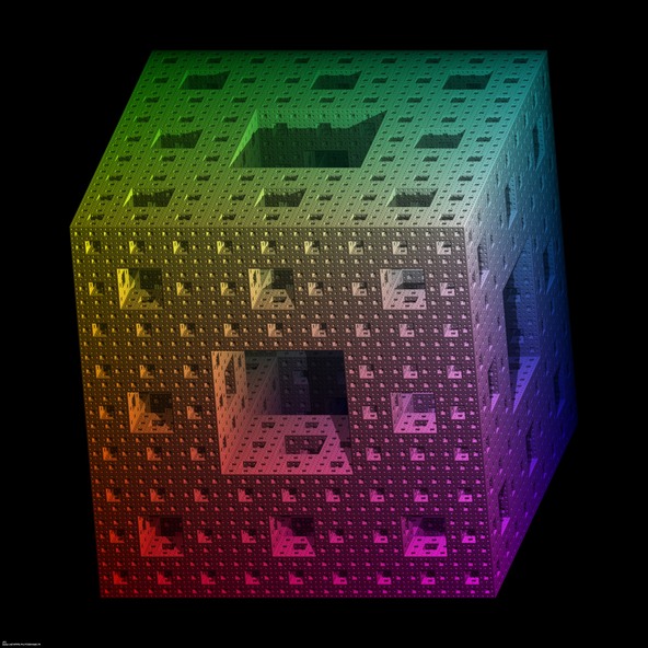
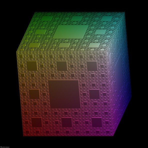
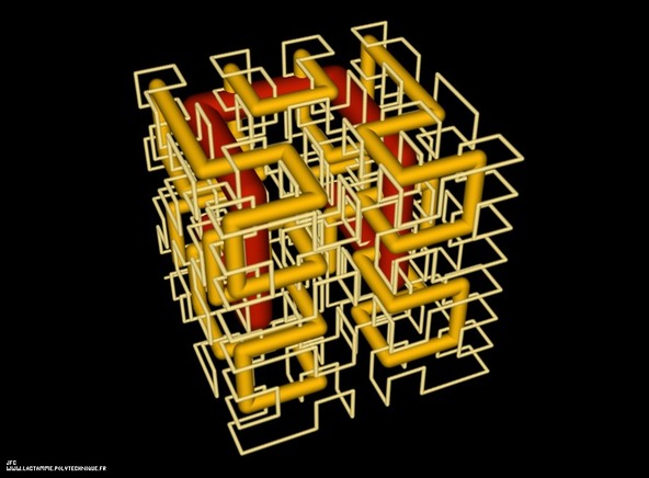
The Menger sponge -iteration 5-.
Definition of the Menger sponge: A cube is cut into 3x3x3=27 identical smaller cubes. Then the 7 central subcubes (6 for each face and 1 at the center of the cube) are removed. At last this process is iterated recursively to the 27-7=20 remaining subcubes. The fractal dimension of the Menger sponge is equal to :
log(20)/log(3) = 2.726833027860842


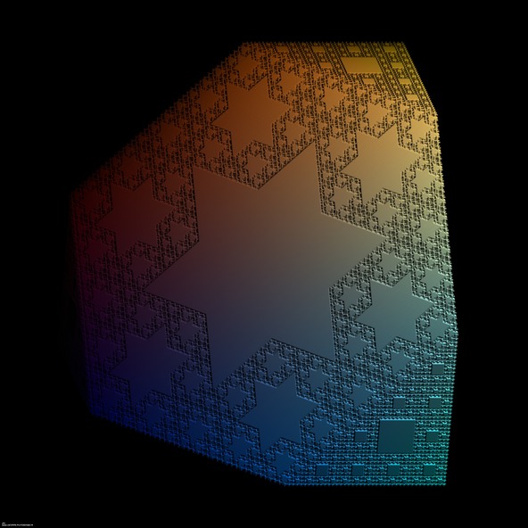
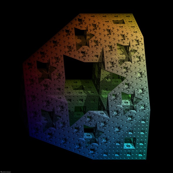
An amazing cross-section inside the Menger sponge -iteration 5-.
Definition of the Menger sponge: A cube is cut into 3x3x3=27 identical smaller cubes. Then the 7 central subcubes (6 for each face and 1 at the center of the cube) are removed. At last this process is iterated recursively to the 27-7=20 remaining subcubes. The fractal dimension of the Menger sponge is equal to :
log(20)/log(3) = 2.726833027860842…
An amazing cross-section can be made using the plane:
2X - 2Y + 2Z - 1 = 0


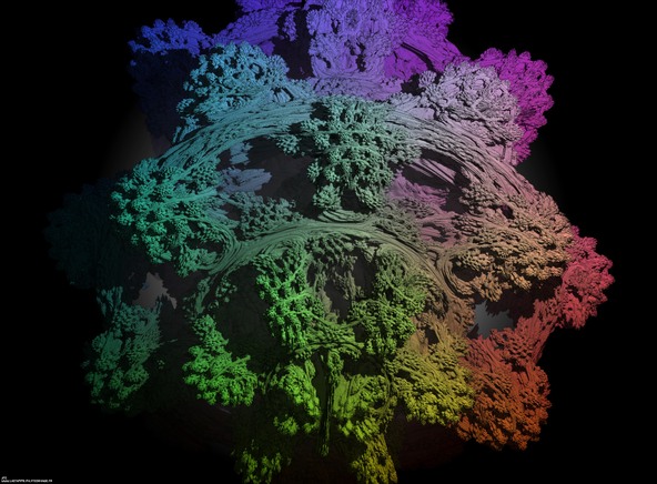
An amazing cross-section inside the Menger sponge -iteration 5- with a (4xO+1)/(1xO-1) conformal transformation in the Octonionic space -tridimensional cross-section-.
Definition of the Menger sponge: A cube is cut into 3x3x3=27 identical smaller cubes. Then the 7 central subcubes (6 for each face and 1 at the center of the cube) are removed. At last this process is iterated recursively to the 27-7=20 remaining subcubes. The fractal dimension of the Menger sponge is equal to :
log(20)/log(3) = 2.726833027860842…
An amazing cross-section can be made using the plane:
2X - 2Y + 2Z - 1 = 0

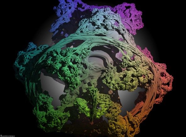
An amazing cross-section inside the Menger sponge -iteration 5- with a 1/O conformal transformation in the Octonionic space -tridimensional cross-section-.
Definition of the Menger sponge: A cube is cut into 3x3x3=27 identical smaller cubes. Then the 7 central subcubes (6 for each face and 1 at the center of the cube) are removed. At last this process is iterated recursively to the 27-7=20 remaining subcubes. The fractal dimension of the Menger sponge is equal to :
log(20)/log(3) = 2.726833027860842…
An amazing cross-section can be made using the plane:
2X - 2Y + 2Z - 1 = 0

The complement of the Menger sponge -iteration 5-.
Definition of the Menger sponge: A cube is cut into 3x3x3=27 identical smaller cubes. Then the 7 central subcubes (6 for each face and 1 at the center of the cube) are removed. At last this process is iterated recursively to the 27-7=20 remaining subcubes.


An amazing cross-section inside the complement of the Menger sponge -iteration 5-.
Definition of the Menger sponge: A cube is cut into 3x3x3=27 identical smaller cubes. Then the 7 central subcubes (6 for each face and 1 at the center of the cube) are removed. At last this process is iterated recursively to the 27-7=20 remaining subcubes.
An amazing cross-section can be made using the plane:
2X - 2Y + 2Z - 1 = 0


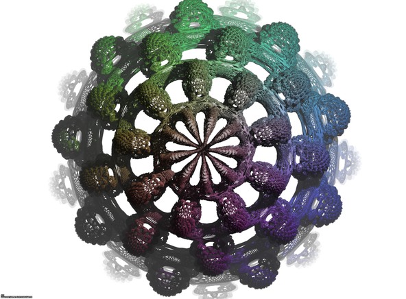
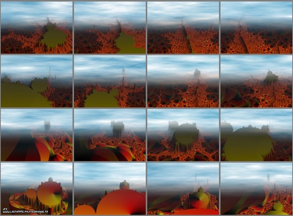
A foggy pseudo-octonionic Julia set ('MandelBulb' like: a 'JuliaBulb') computed with A=(-0.58...,+0.63...,0,0,0,0,0,0) with a rotation about the X axis -tridimensional cross-section-.
See http://www. lactamme. polytechnique.fr/Mosaic/descripteurs/NDimensionalDeterministicFractalSets.01.Ang.html for more information about this subject.


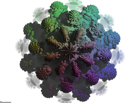
A foggy pseudo-octonionic Julia set computed with A=(-0.58...,+0.63...,0,0,0,0,0,0) with a rotation about the X axis -tridimensional cross-section-.
See http://www. lactamme. polytechnique.fr/Mosaic/descripteurs/NDimensionalDeterministicFractalSets.01.Ang.html for more information about this subject.


A foggy pseudo-octonionic Julia set computed with A=(-0.58...,+0.63...,0,0,0,0,0,0) with a rotation about the X axis -tridimensional cross-section-.
See http://www. lactamme. polytechnique.fr/Mosaic/descripteurs/NDimensionalDeterministicFractalSets.01.Ang.html for more information about this subject.


A foggy pseudo-octonionic Julia set computed with A=(-0.58...,+0.63...,0,0,0,0,0,0) -tridimensional cross-section-.
See http://www. lactamme. polytechnique.fr/Mosaic/descripteurs/NDimensionalDeterministicFractalSets.01.Ang.html for more information about this subject.


A foggy pseudo-octonionic Julia set computed with A=(-0.58...,+0.63...,0,0,0,0,0,0) -tridimensional cross-section-.
See http://www. lactamme. polytechnique.fr/Mosaic/descripteurs/NDimensionalDeterministicFractalSets.01.Ang.html for more information about this subject.


A foggy pseudo-octonionic Julia set computed with A=(-0.58...,+0.63...,0,0,0,0,0,0) -tridimensional cross-section-.
See http://www. lactamme. polytechnique.fr/Mosaic/descripteurs/NDimensionalDeterministicFractalSets.01.Ang.html for more information about this subject.


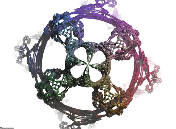
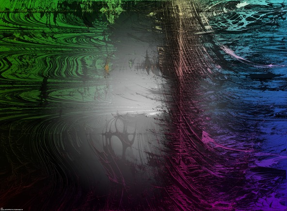
A pseudo-octonionic Mandelbrot set -tridimensional cross-section-.
See http://www. lactamme. polytechnique.fr/Mosaic/descripteurs/NDimensionalDeterministicFractalSets.01.Ang.html for more information about this subject.


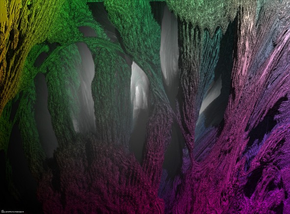
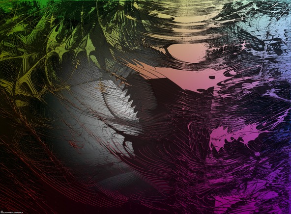
Close-up on a pseudo-octonionic Mandelbrot set -tridimensional cross-section-.
See http://www. lactamme. polytechnique.fr/Mosaic/descripteurs/NDimensionalDeterministicFractalSets.01.Ang.html for more information about this subject.


A tribute to Benoît Mandelbrot (1924-2010): tridimensional zoom in on the Mandelbrot set with mapping of the arguments.


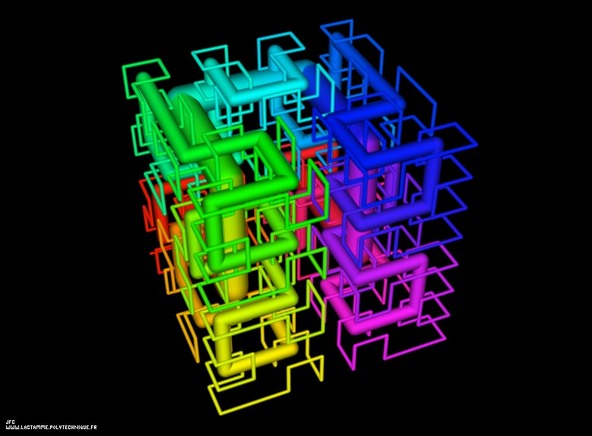
Tridimensional visualization of the Verhulst dynamics
The Verhulst dynamics is defined using the following iteration:
X[0] = 0.5
X[n] = R.X[n-1].(1 - X[n-1])
Here, in this computation, the growing rate ‘R’ is no longer constant but changes its value periodically using the following arbitrary cycle:
R3 ==> R3 ==> R2 ==> R1 ==> R2 ==> R3 ==> R1 ==> R2 ==> R3 ==> R1 ==> R1 ==> R1
where {R1,R2,R3} are respectively the three coordinates of the current point inside the following domain [2.936,3.413]x[3.500,3.850]x[3.000,4.000].
Only the points corresponding to a dynamical system with a negative Lyapunov exponent are displayed.


Tridimensional visualization of the Verhulst dynamics
The Verhulst dynamics is defined using the following iteration:
X[0] = 0.5
X[n] = R.X[n-1].(1 - X[n-1])
Here, in this computation, the growing rate ‘R’ is no longer constant but changes its value periodically using the following arbitrary cycle:
R3 ==> R3 ==> R2 ==> R2 ==> R1 ==> R1 ==> R2 ==> R2 ==> R1 ==> R1 ==> R2 ==> R3 ==> R2 ==> R1 ==> R1 ==> R1where {R1,R2,R3} are respectively the three coordinates of the current point inside the following domain [2.936,3.413]x[3.500,3.850]x[3.000,4.000].
Only the points corresponding to a dynamical system with a negative Lyapunov exponent are displayed.


Tridimensional visualization of the Verhulst dynamics
The Verhulst dynamics is defined using the following iteration:
X[0] = 0.5
X[n] = R.X[n-1].(1 - X[n-1])
Here, in this computation, the growing rate ‘R’ is no longer constant but changes its value periodically using the following arbitrary cycle:
R3 ==> R3 ==> R3 ==> R3 ==> R3 ==> R3 ==> R3 ==> R3 ==> R2 ==> R2 ==> R2 ==> R2 ==> R2 ==> R2 ==> R1 ==> R1 ==> R1 ==> R1 ==> R1 ==> R1 ==> R1 ==> R1 ==> R1 ==> R2 ==> R2 ==> R2 ==> R3 ==> R3 ==> R3 ==> R3 ==> R2 ==> R2 ==> R2 ==> R1 ==> R1 ==> R1 ==> R1 ==> R1 ==> R1 ==> R1 ==> R2 ==> R2 ==> R2 ==> R3 ==> R3 ==> R3 ==> R3 ==> R3 ==> R2 ==> R2 ==> R2 ==> R2 ==> R1 ==> R1 ==> R1 ==> R1 ==> R1 ==> R1 ==> R1 ==> R1 ==> R1 ==> R1 ==> R1 ==> R1where {R1,R2,R3} are respectively the three coordinates of the current point inside the following domain [2.936,3.413]x[3.500,3.850]x[3.000,4.000].
Only the points corresponding to a dynamical system with a negative Lyapunov exponent are displayed.


Tridimensional visualization of the Verhulst dynamics
Tridimensional visualization of the Verhulst dynamics
The Verhulst dynamics is defined using the following iteration:
X[0] = 0.5
X[n] = R.X[n-1].(1 - X[n-1])
Here, in this computation, the growing rate ‘R’ is no longer constant but changes its value periodically using the following arbitrary cycle:
R5 ==> R5 ==> R5 ==> R5 ==> R5 ==> R5 ==> R5 ==> R4 ==> R4 ==> R4 ==> R4 ==> R3 ==> R3 ==> R2 ==> R2 ==> R1 ==> R1 ==> R1 ==> R1 ==> R1 ==> R1 ==> R2 ==> R2 ==> R3 ==> R3 ==> R4 ==> R4 ==> R5 ==> R5 ==> R4 ==> R4 ==> R3 ==> R2 ==> R2 ==> R1 ==> R1 ==> R1 ==> R1 ==> R1 ==> R2 ==> R3 ==> R3 ==> R4 ==> R4 ==> R5 ==> R5 ==> R5 ==> R4 ==> R4 ==> R4 ==> R3 ==> R3 ==> R2 ==> R2 ==> R1 ==> R1 ==> R1 ==> R1 ==> R1 ==> R1 ==> R1 ==> R1 ==> R1 ==> R1where {R1,R2,R3,R4,R5} are respectively the five coordinates of the current point inside the following domain [2.936,3.413]x[3.500,3.850]x[3.000,4.000]x[2.7]x[2.9]. Only the points corresponding to a dynamical system with a negative Lyapunov exponent are displayed.


Tridimensional visualization of the Verhulst dynamics
The Verhulst dynamics is defined using the following iteration:
X[0] = 0.5
X[n] = R.X[n-1].(1 - X[n-1])
Here, in this computation, the growing rate ‘R’ is no longer constant but changes its value periodically using the following arbitrary cycle:
R3 ==> R3 ==> R3 ==> R3 ==> R2 ==> R2 ==> R2 ==> R1 ==> R1 ==> R1 ==> R1 ==> R2 ==> R2 ==> R3 ==> R3 ==> R2 ==> R1 ==> R1 ==> R1 ==> R1 ==> R2 ==> R2 ==> R3 ==> R3 ==> R2 ==> R2 ==> R1 ==> R1 ==> R1 ==> R1 ==> R1 ==> R1where {R1,R2,R3} are respectively the three coordinates of the current point inside the following domain [2.936,3.413]x[3.500,3.850]x[3.000,4.000]. Only the points corresponding to a dynamical system with a negative Lyapunov exponent are displayed.


Tridimensional visualization of the Verhulst dynamics
The Verhulst dynamics is defined using the following iteration:
X[0] = 0.5
X[n] = R.X[n-1].(1 - X[n-1])
Here, in this computation, the growing rate ‘R’ is no longer constant but changes its value periodically using the following arbitrary cycle:
R1 ==> R2 ==> R3 ==> R1 ==> R1 ==> R2 ==> R2 ==> R3 ==> R3 ==> R1 ==> R1 ==> R1 ==> R2 ==> R2 ==> R2 ==> R3 ==> R3 ==> R3 ==> R1 ==> R1 ==> R1 ==> R1 ==> R2 ==> R2 ==> R2 ==> R2 ==> R3 ==> R3 ==> R3 ==> R3where {R1,R2,R3} are respectively the three coordinates of the current point inside the following domain [2.936,3.413]x[3.500,3.850]x[3.000,4.000]. Only the points corresponding to a dynamical system with a negative Lyapunov exponent are displayed.


Tridimensional visualization of the Verhulst dynamics
The Verhulst dynamics is defined using the following iteration:
X[0] = 0.5
X[n] = R.X[n-1].(1 - X[n-1])
Here, in this computation, the growing rate ‘R’ is no longer constant but changes its value periodically using the following arbitrary cycle:
R1 ==> R2 ==> R3 ==> R1 ==> R1 ==> R2 ==> R2 ==> R3 ==> R3 ==> R1 ==> R1 ==> R1 ==> R2 ==> R2 ==> R2 ==> R3 ==> R3 ==> R3 ==> R1 ==> R1 ==> R1 ==> R1 ==> R2 ==> R2 ==> R2 ==> R2 ==> R3 ==> R3 ==> R3 ==> R3where {R1,R2,R3} are respectively the three coordinates of the current point inside the following domain [3.212,3.370]x[3.500,3.616]x[3.000,4.000]. Only the points corresponding to a dynamical system with a negative Lyapunov exponent are displayed.


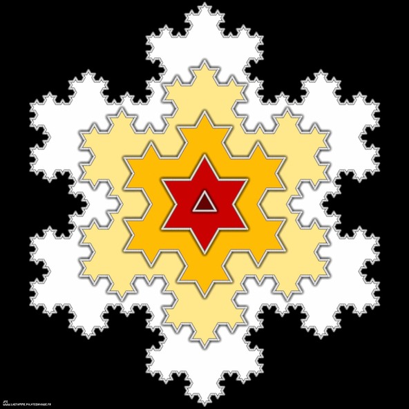
Tridimensional view of the first four iterations of the construction of the von Koch snowflake
(제목번역: 코흐 곡선의 첫 4단계 반복의 3차원 조망)


The first four iterations of the construction of the von Koch snowflake
(제목번역: 코흐 곡선의 첫 4단계 반복)


