Colorful Brownian Motion
program
Licenses
Source code
Website
With this web demo, you can play around with and learn something about Brownian Motion, a fundamental concept in the theory of stochastic processes and probabilistic physics.
What is Brownian Motion?
Brownian Motion is pretty cool! Imagine a random walk in some space. Maybe you have a point on a plane, it moves one step right, left, up and down with probability 1/4 each. You can do interesting things with that process, for example think about whether it comes back to its original position (it does, by the way). What makes it fundamentally different from our world though is, that we live in continuous time. In our world, things move smoothly. So wouldn’t it be kind of neat to have a process like the random walk, but in continuous time? Well, that process is Brownian motion. In the simulation above, you can see something that… isn’t Brownian motion. As you can imagine, computers aren’t very good at computing infinitely many time steps. But as you decrease the “variance” slider, you can see what kind of process we are talking about. Brownian motion was first described in written form when a guy called Robert Brown peeked into his microscope to look at his favourite small, lightweight object on a fluid and noticed that it was all jittery. Jittery, you will have noticed, as the simulation above.
What’s up with the colors?
The fun thing is that Brownian Motion can happen in any space similar to the real numbers - if you want it to. So here, it happens in the x-y-Plane and a subsection of the RGB color space. Numerically, at each time step, all five coordinates get an increment drawn out of a centered normal distribution with variance as specified by you.
And you can do maths with this?
Yes! It’s not that easy though, at least to me it’s not obvious why a process with normally distributed, independent increments and (almost surely) continuous paths would even exist. With some background in measure theory you can find out a few interesting things though, for example give confidence bands of where the process is likely to be for increasing time. The intuition is that going straight for a long time is very unlikely, therefore the process tends to stay where it started. Turns out, it only moves away from its starting point proportionally to the sqare root of the elapsed time, which is a pretty useful result! After all, this models real things also, like small particles in a fluid. (Note that this only applies to the above simulation as long as it doesn’t touch the border.)


