A few examples of stochastic processes from physics and biology
The images in this gallery are mostly simulations of stochastic processes, arising from applications in statistical physics or in biology. A stochastic process is a process evolving in time in a random way. Thus it can also be seen as a family of random variables indexed by time. Typical examples are the size of a population, the boundary between two phases in an alloy, or interacting molecules at positive temperature.
The programs generating these images have been coded directly in C, which is used to produce eps files, which can then be translated into other formats. There are also a couple of related movies in the films section.
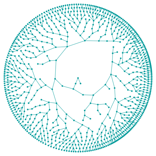
Galton-Watson tree
A realisation of a Galton-Watson tree. The ancestor, in the center of the picture, has two children. Each individual has again a random number of children (between 0 and 3 in this simulation), all children numbers being independent and identically distributed.
Une réalisation d’un arbre de Bienaymé-Galton-Watson. L’ancêtre, au centre de l’image, a deux enfants. Chaque individu a à nouveau un nombre aléatoire d’enfants (entre 0 et 3 dans cette simulation), tous les nombres d’enfants étant indépendants et identiquement distribués.
Pour une explication détaillée, voir http://images. math. cnrs.fr/La-probabilite-d-extinction-d-une.html

Bond percolation
A realisation of bond percolation on a subset of Z2 (p = 0.525).
Each edge is open with probability p. Dark edges form the connected component of the lower boundary.
Une réalisation d’une percolation de lien sur une partie de Z2 (p = 0.525).
Chaque lien est ouvert avec probabilité p. Les liens foncés forment la composante connexe du bord inférieur.
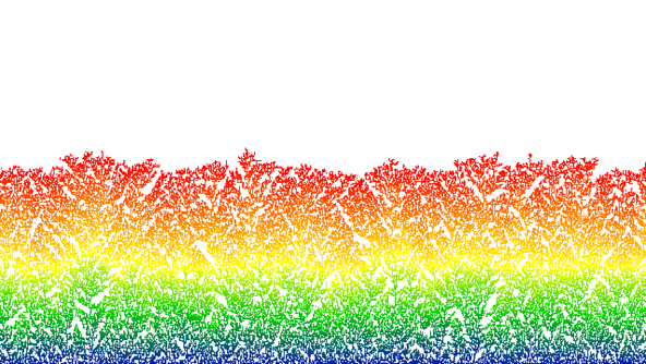
Surface growth model
Particles fall randomly and get stuck as soon as they touch another particle below or sideways. The scaling limit of this model is governed by the KPZ equation.
Des particules tombent de manière aléatoire et restent figées dès qu’elles touchent une autre particule en dessous ou sur les côtés. La limite d’échelle de ce modèle est gouvernée par l’équation KPZ.
Voir aussi http://images. math. cnrs.fr/Qu-est-ce-qu-une-Equation-aux.html

Stochastic Allen-Cahn equation
The stochastic Allen-Cahn equation describes phase separation in an alloy.
L’équation d’Allen-Cahn stochastique décrit la séparation de phases dans un alliage.
Voir aussi http://images. math. cnrs.fr/Qu-est-ce-qu-une-Equation-aux.html

Bernoulli site percolation on a square lattice
Benoulli site percolation on a square lattice of size 992 x 1920. Each site is open with probability 0.5997, and closed otherwise, independently of all other sites. Closed sites are shown in yellow. Open sites connected to the left boundary are shown in purple, the other open sites in cyan. The critical value of Bernoulli site percolation on a square lattice is approximately 0.59274. Beyond this value, as the lattice size goes to infinity, there is an infinite open cluster with probability 1. Below this value, the probability is 0.
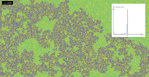
Bernoulli bond percolation on a square lattice
Benoulli bond percolation on a square lattice of size 992 x 1920. Each site is open with probability 0.4993, and closed otherwise, independently of all other sites. Closed sites are shown in yellow. Open sites connected to the left boundary are shown in blue, the other open sites in cyan. The critical value of Bernoulli site percolation on a square lattice is equal to 1/2. Beyond this value, as the lattice size goes to infinity, there is an infinite open cluster with probability 1. Below this value, the probability is 0.

Bernoulli percolation on a honeycomb lattice
Benoulli percolation on a honeycomb lattice of size 71 x 119. Each hexagon is open with probability 0.4823, and closed otherwise, independently of all other hexagons. Closed hexagons are shown in blue. Open hexagons connected to the left boundary are shown in yellow, the other open hexagons in gray. The critical value of Bernoulli percolation on a honeycomb lattice is equal to 1/2. Beyond this value, as the lattice size goes to infinity, there is an infinite open cluster with probability 1. Below this value, the probability is 0.

Percolation clusters near criticality on a honeycomb lattice
Clusters of Bernoulli site percolation on a honeycomb lattice. Connected open components are shown in different colors. The probability that a bond is open is equal to 0.4978.
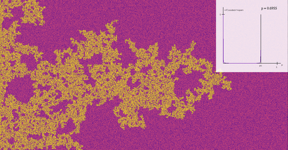
Bernoulli site percolation on a lattice of triangles
The cells of the lattice are equilateral triangles. Their centers form a hexagonal lattice, whose Voronoi cells are the triangles.
The parameter p = 0.6955 is the probability that a triangle is open. Closed triangles are shown in purple, and open ones in yellow when they are connected to the left boundary, and pink otherwise. The increase of p slows down when it reaches the critical value, which is approximately equal to 0.69704. The graph shows the rsize of the percolation cluster (the set of open triangles connected to the left boundary), divided by the number of open triangles, as a function of p.
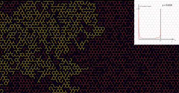
Bernoulli bond percolation on a honeycomb lattice
The parameter p increasing from 0 to 1 is the probability that a bond is open. Closed bonds are shown in dark purple, and open ones in yellow when they are connected to the left boundary, and pink otherwise. The increase of p slows down when it reaches the critical value, which is equal to 1 - 2*sin(Pi/18), or about 0.652703645. The graph shows the rsize of the percolation cluster (the set of open bonds connected to the left boundary), divided by the number of open bonds, as a function of p.
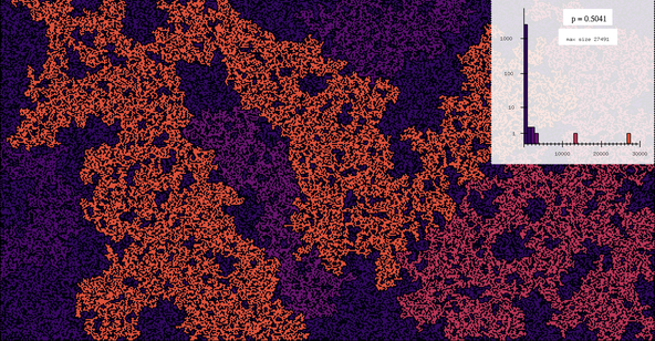
Percolation clusters near criticality on a honeycomb lattice
Clusters of Bernoulli site percolation on a honeycomb lattice. Connected open components are shown in different colors. The probability that a bond is open is equal to 0.5041.

Percolation clusters near criticality on a lattice of triangles
Clusters of a percolation configuration on a lattice of triangles (whose centers form a hexagonal lattice). The probability of a triangle to be open is equal to 0.69704, which is close to the numerically determined critical value. The clusters are therefore statistically self-similar.

